Solution Verification
Solution verification
Solution verification can be carried out by analyzing model results on progressively refined meshes. The two main indicators to assess mesh convergence are the Relative Discretization Error (RDE) 1 and the Richardson extrapolation. The latter is mostly used in Computation Fluid Dynamics, and assumes that the model is in the asymptotic range regarding the mesh size. In 2, it is shown that using four meshes allows to estimate the confidence in Richardson extapolation.
Note
The time (for explicit models) or pseudo-time integration scheme could also be verified.
These two methods are implemented in VIMSEO, in the tool named DiscretizationSolutionVerification.
and can be displayed by the dashboard dashboard_verification.
Solution verification is performed through a convergence study of the solution
on four progressively refined meshes (only three meshes would be strictly necessary),
which allows to compute some uncertainties on the \(GCI\), RDE and
Richardson extrapolation.
An example of Python script setting up the solution verification for the OpfmPlate model with load case PST
can be found
here.
Mesh Convergence Indicators
Several indicators are used to help decision-making on the approriate mesh element size.
Notations
\(\gamma_0\) to \(\gamma_3\) are element sizes, from coarsest to finest. \(q_{\gamma_i}\) is the solution obtained on the mesh with element size \(\gamma_i\). \(E_q = q_{exact} - q_{\gamma}\) is the true error of the solution.
Richardson extrapolation
Considering \(\gamma\) is a continuous variable, the true error on the simulation result \(q\) can be expanded in \(\gamma\):
\(\beta\) can be obtained by solving a non-linear equation involving solutions on three progressively refined meshes. Note that a solution for \(\beta\) cannot always be found.
Once \(\beta\) is found, \(C\) can be obtained by considering the solution on two meshes (by subtracting the above equation, which cancels \(q_{exact})\). Finally, the Richardson extrapoled value \(q_{exact}\) can be computed from \(C\) and \(\beta\).
Grid Convergence Index
The \(GCI\) is an indicator of the solution convergence on the mesh. It requires to know the order of convergence of the solution, based on the computation of the extrapoled value with Richardson method. The \(GCI\) requires the solution on two meshes. Thus different values for the \(GCI\) can be obtained from four meshes. For the two fines meshes, the \(GCI\) is:
An error band can be computed for the \(GCI\)2:
\(E_b(GCI_{finest}) = q_{\gamma_3} (1 \pm GCI_{finest})\)
However, it is often the case that Richardson extrapolation cannot be computed (for instance, if the solution oscillates between consecutive refined meshes). In such case, we can still provide a value of the \(GCI\) by assuming a convergence order. Note also that two meshes must be selected to compute this indicator. Currently, the \(GCI\) is computed on the two finest meshes and the two coarsest meshes. The solution verification dashboard shows these two \(GCI\) values for:
- the computed order of convergence, if possible
- an assumed order of convergence of one and two.
Relative Discretization Error
The RDE is another indicator of the numerical error due to the mesh discretization. It can be computed from two meshes. Thus three RDE values can be computed from the four simulated meshes. Note that it also requires that the extrapolated value with Richardson method is computed.
and similarly as for the \(GCI\):
\(E_b(RDE) = q_{\gamma_3} (1 \pm RDE)\)
TODO: refer to vimseo doc once ported to mkdocs and deployed
TODO: add a synthetic uncertainty indicator, that can be used for decision making.
Element size choice
At least three progressively refined meshes are necessary to compute the above indicators.
According to 2,
running four meshes allows to get some confidence intervals
on the indicators.
The DiscretizationSolutionVerification implements this approach, where
four element sizes must be specified in strictly decreasing order.
In the following application, the element sizes are \([dx_0 \times r, dx_0, dx_0 \times r^{-1}, dx_0 \times r^{-2}]\). They become \([CF \times r, CF, CF \times r^{-1}, CF \times r^{-2}]\) if the model input controlling the mesh size is the \(coarsening\_factor\) (\(CF\)). We choose \(r=1.2\).
Note
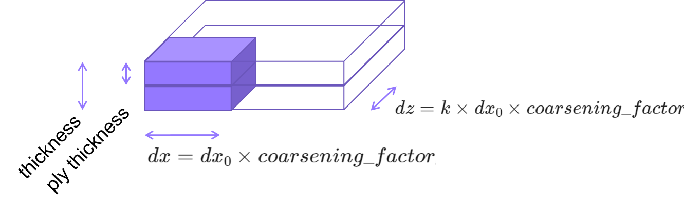
Some models have their element size controlled by the input
coarsening_factor. The relationship with the element size \(dx\) is
\(dx = dx_0 \times coarsening\_factor\),
with \(dx_0\) is the nominal element size.
-
Christopher J. Roy. Review of code and solution verification procedures for computational simulation. Journal of Computational Physics, 205(1):131–156, 2005. URL: https://www.sciencedirect.com/science/article/pii/S0021999104004619, doi:https://doi.org/10.1016/j.jcp.2004.10.036. ↩
-
Petr Krysl. Confidence intervals for richardson extrapolation in solid mechanics. J. Verif. Valid. Uncert., 7(3):031005, 2022. doi:https://doi.org/10.1115/1.4055728. ↩↩↩