Code verification opfm

Verification of the Opfm material law¶

TODO replace OpfmCUbe by OpfmUnitcell

To verify that the expected model form is correctly implemented, the OpfmCube model is used. Indeed, this model uses the same run-processor processor component (and thus the same material subroutine) as the OpfmPlate model. It differs from the latter by its pre-processor and post-processor components, in which an RVE approach is used instead of a meshed model of a plate. Thus, it allows the verification of the implementation of the model dataflow, the call to Abaqus with proper options, and the interfacing with the subroutine. The verification is based on the relationship between the material properties defined as inputs and the model's outputs such as max_strength. For instance, when considering the response simulated with the OpfmCube model under a pure longitudinal load (PST on 0° laminate), the material property Xt should be equal to the max_strength output. The code verification relies on the VIMSEO CodeVerificationAgainstData tool, where an example is given here.

The error between Xt and max_strength is computed for two values of the numerical parameter nb_intervals, which controls the convergence of the subroutine. The reference dataset that needs to be specified to the CodeVerificationAgainstData tool is composed of three variables: - the inputs Xt and nb_intervals - the output max_strength

Several metrics of comparison can be specified to evaluate the error between the reference output and the corresponding simulated value.

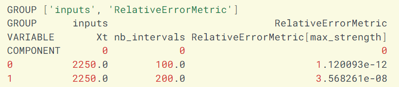
Here, the relative error is found to be negligible.

Matrix¶

Unnamed: 1	Unnamed: 2	Unnamed: 3	Unnamed: 4
OpfmPlate	OpfmUnitCell	OpfmCube	rel_tol
PST, [0]	PST0	PST0	0.2
PST, [0, 0]	PST0	PST0	0.2
PST, [90]	PST90	PST90	0.2
PST, [90, 90]	PST90	PST90	0.2
PSC, [0]	PSC0	PSC0	0.2
PSC, [0, 0]	PSC0	PSC0	0.2
PSC, [90]	PSC90	PSC90	0.2
PSC, [90, 90]	PSC90	PSC90	0.2
PST, [45, -45]s	IPS	IPS	0.2
nan	nan	nan	nan
nan	nan	nan	nan
PgPlate	nan	nan	nan
OHT	VATool	nan	0.2
PST	VATool	nan	0.2
nan	nan	nan	nan
nan	nan	nan	nan
nan	nan	nan	nan
OpfmCube	nan	nan	nan
PST0	max_strength=Xt	nan	epsilon
PSC0	max_strength=Xc	nan	epsilon
PST90	max_strength=Yt	nan	epsilon
PSC90	max_strength=Yc	nan	epsilon

Verification of the integration of the Opfm material law with Abaqus¶

Repeat above verif for OpfmCUbe

Then, the integration of the Opfm law with Abaqus, which is done through VIMSEO RunAbaqusWrapper can be performed. First, we can check that the OpfmCube and OpfmUnitCell models return results that are close on load cases with uniform stress distribution. By close, we mean \(10 \%\) error, because the boundary conditions between the two models are not strictly the same.

TODO add link to deployed doc

Code verification for OpfmPlate model PST¶

Secondly, we can check that the OpfmPlate and OpfmCube model also return close results.

The following test matrix is used:

OpfmPlate	layup	OpfmUnitCell	OpfmCube	rel_tol
PST	[0]	PST0	PST0	0.1
PST	[0, 0]	PST0	PST0	0.1
PST	[90]	PST90	PST90	0.1
PST	[90, 90]	PST90	PST90	0.1
PSC	[0]	PSC0	PSC0	0.1
PSC	[0, 0]	PSC0	PSC0	0.1
PSC	[90]	PSC90	PSC90	0.1
PSC	[90, 90]	PSC90	PSC90	0.1

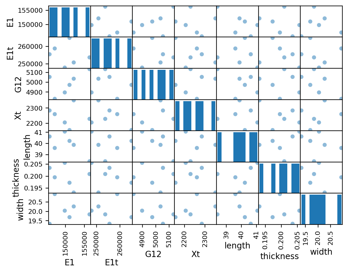
The OpfmPlate PST model is verified against OpfmCube PST. The variables of the parameter space on which the models are sampled correspond to input variables to which the max_strength output is the most sensitive for the OpfmCube PST model, which are:

\(E1\)
\(E1t\)
\(G12\)
\(Xt\)

The geometrical parameters:

\(width\)
\(length\)
\(thickness\)

are also added. Triangular distributions are defined for each variable, ranging over the bounds defined in the Opfm material of vims-composites.

TODO link to example

Layup \([0]\)¶

The input parameter space is represented in the following figure:

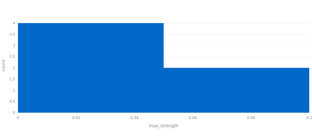
One way to represent how the error range and their distribution is to plot a histogram of the errors (one for each error metric). Thus, in abscissa we have error band values, and in ordinate we have the number of error values within a given band. We observe that the relative error on \(max\_strength\) between the two models can reach \(10 \%\):