Sensitivity
Results for OpfmCube
The results for the OpfmCube model are presented based on the sensitivity viewer dashboard,
which can be obtained by typing dashboard_sensitivity in a console where VIMSEO is installed:
OpfmCube PST
Layup \([30, 90, -30, 90, -30, -30, 90, -30, 90, 30]\)
We present the plots available in the dashboard_sensitivity.
These plots are specialized for a Morris analysis.
Other type of sensitivity analysis would be visualized through
specific plots.
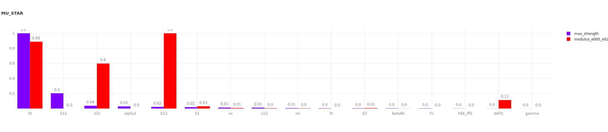
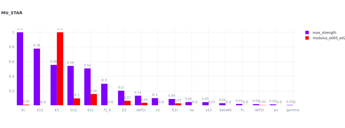
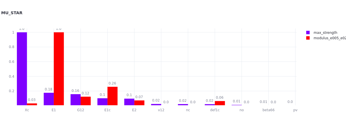
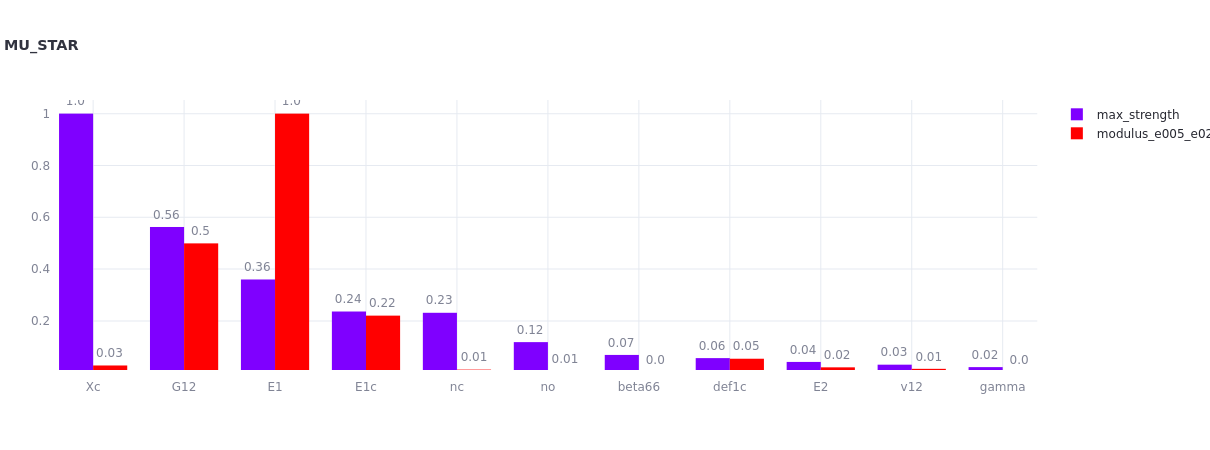
First, a bar plot summarizes the sensitivity of one or several outputs
to all inputs. A standardize option can be used to scale
the highest sensitivity to one. For a Morris analysis,
the \(\mu^*\) indicator is shown.
| \(cov=5 \%\) |
|---|
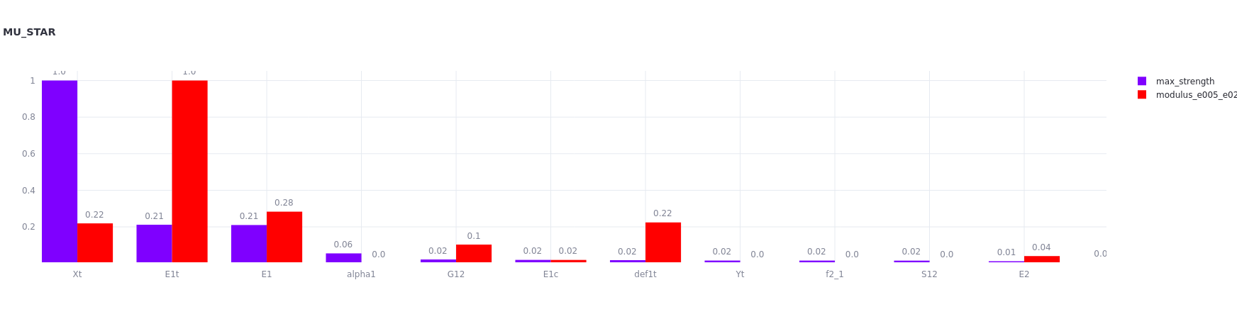 |
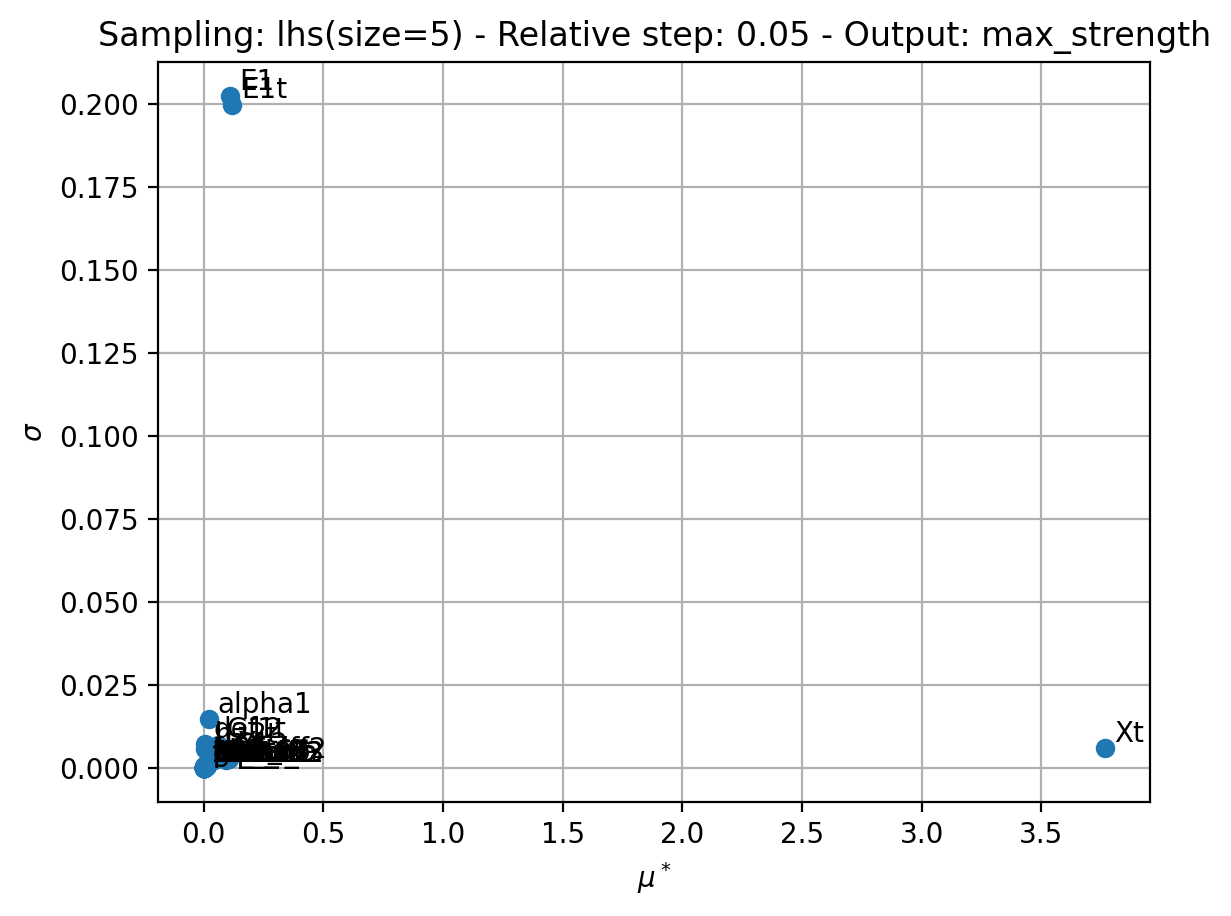
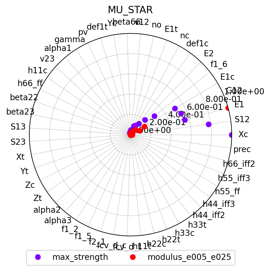
A radar plot representation for \(\mu^*\) index is also available. Based on the max strength, the most sensitive variables are \(X_t\), \(E_{1t}\) and \(E_1\).
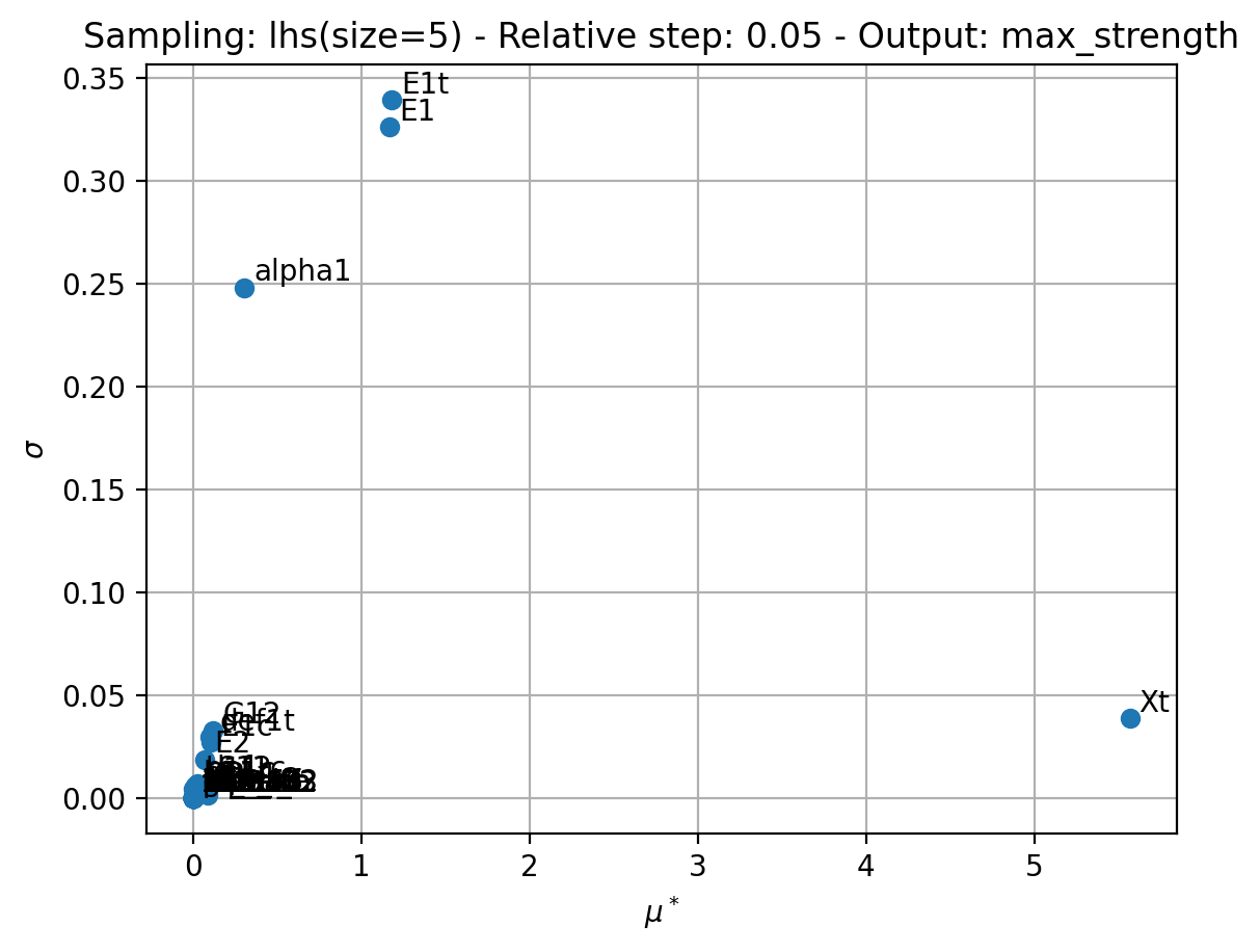
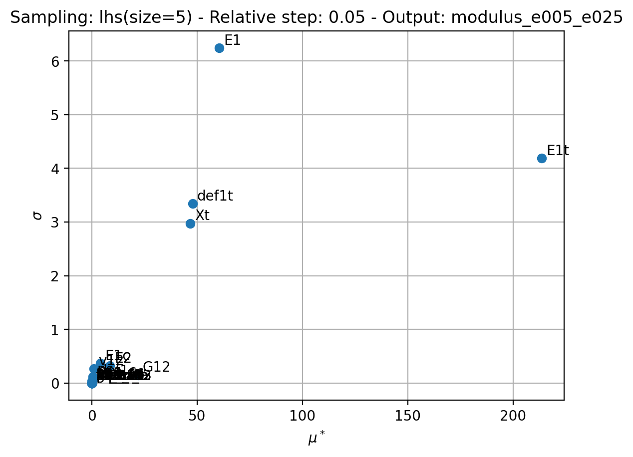
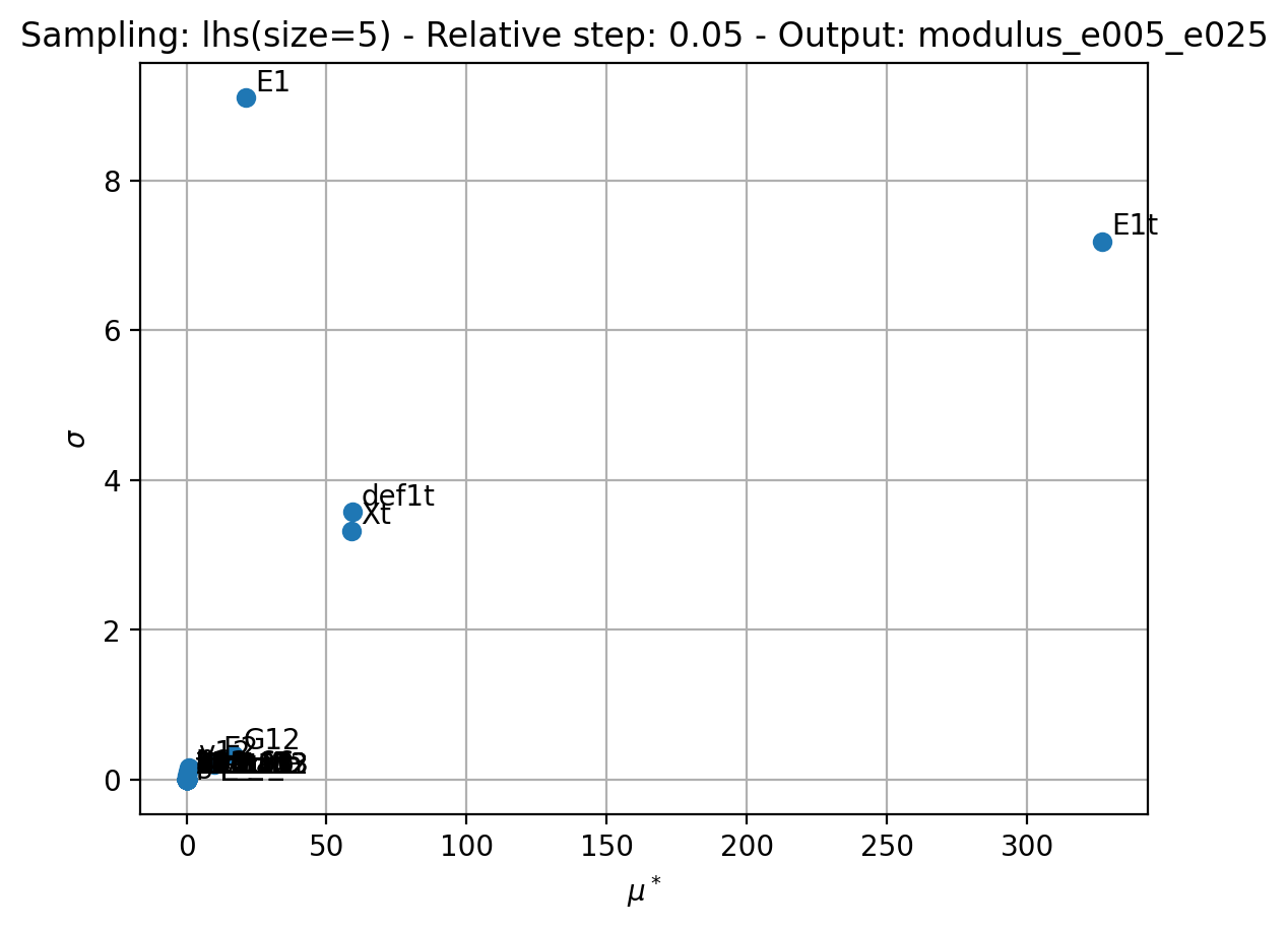
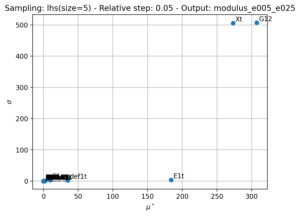
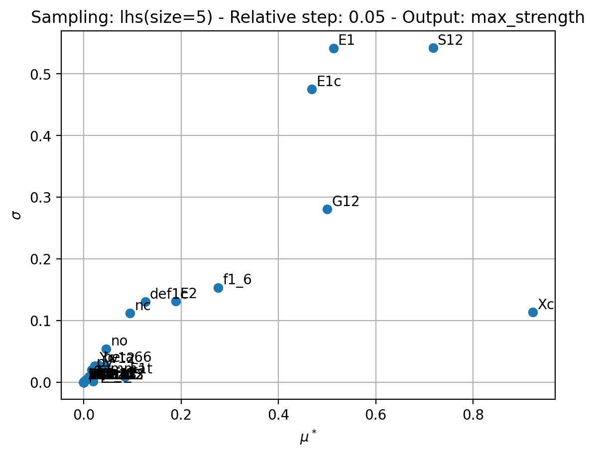
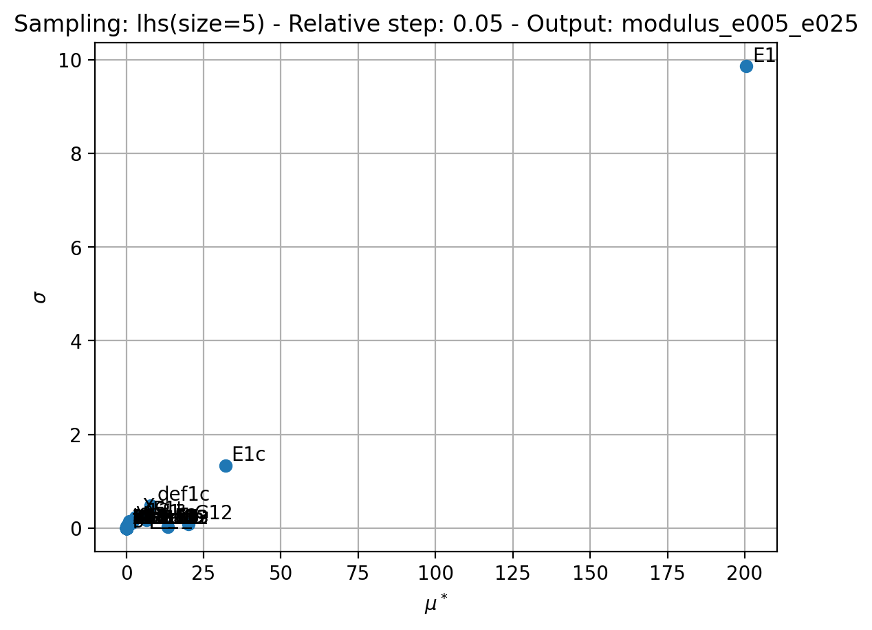
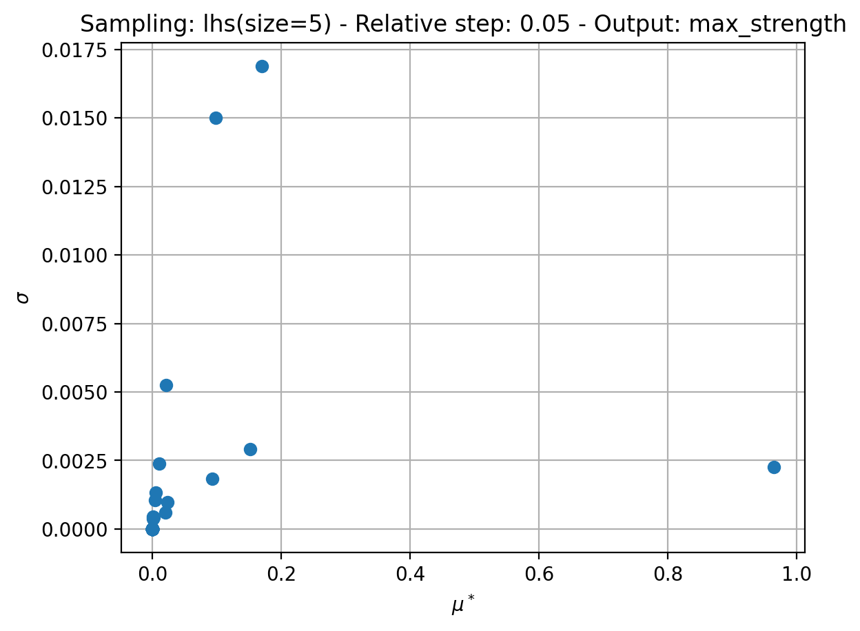
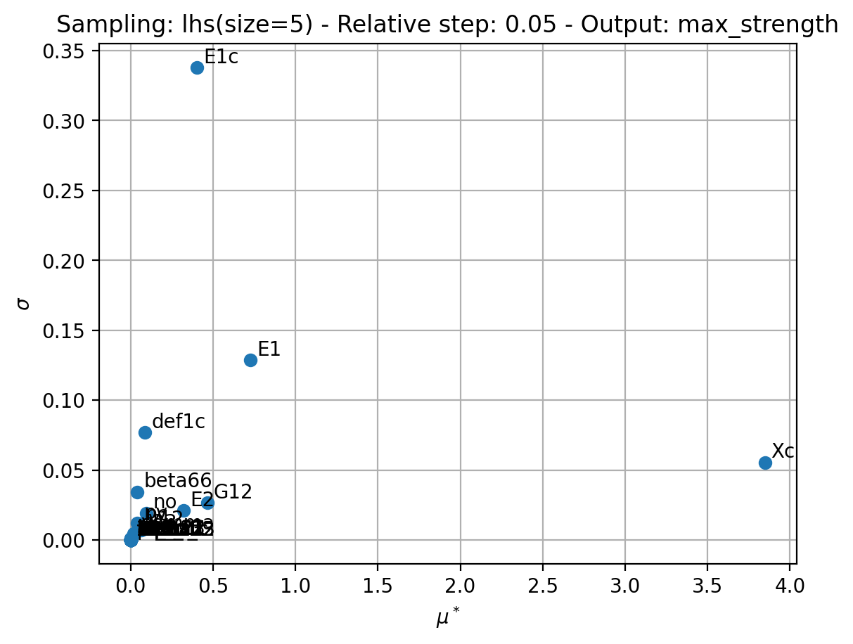
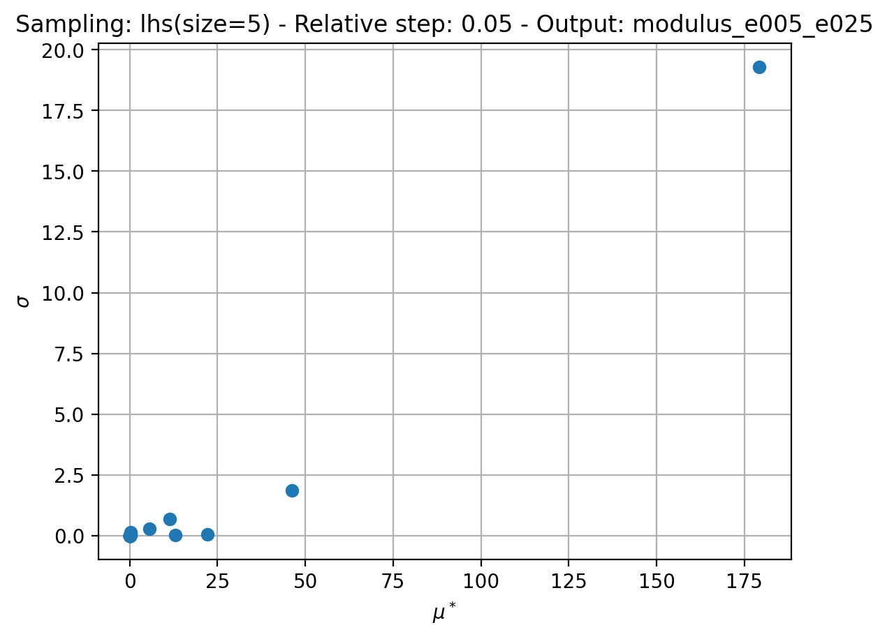
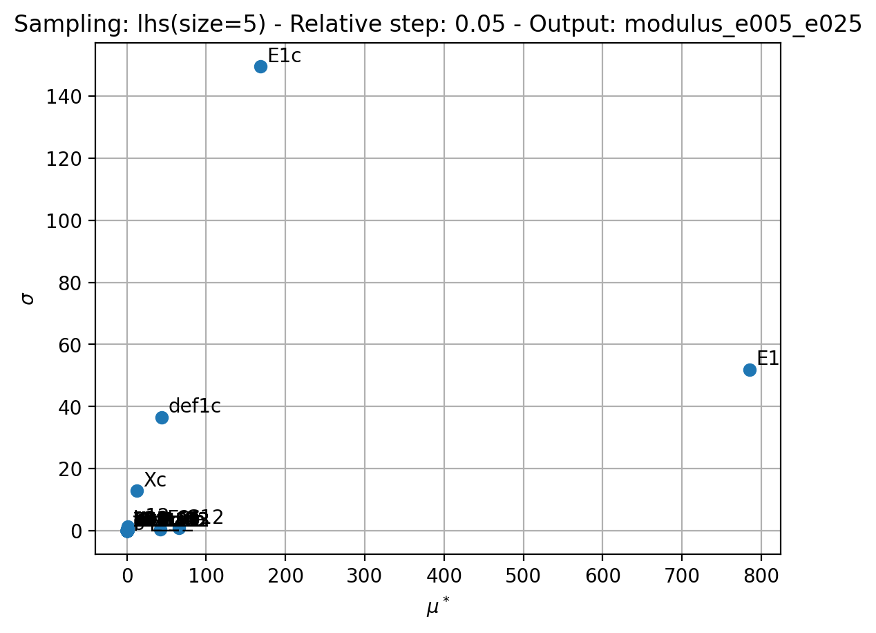
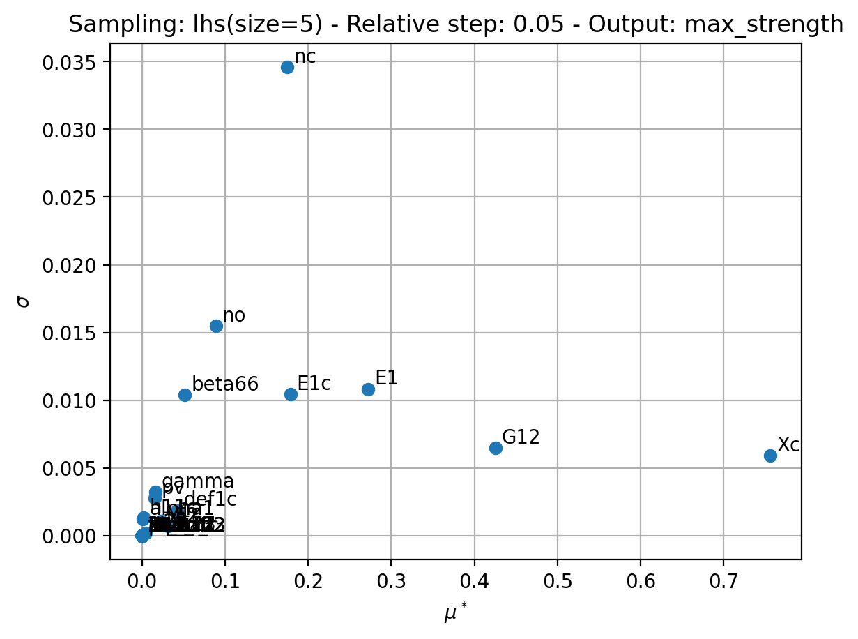
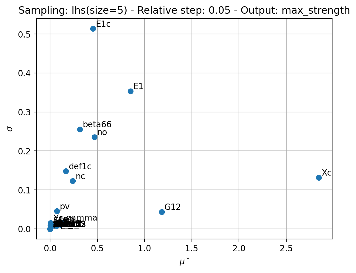
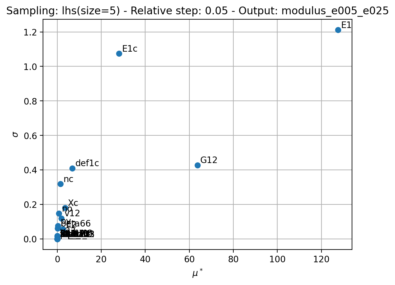
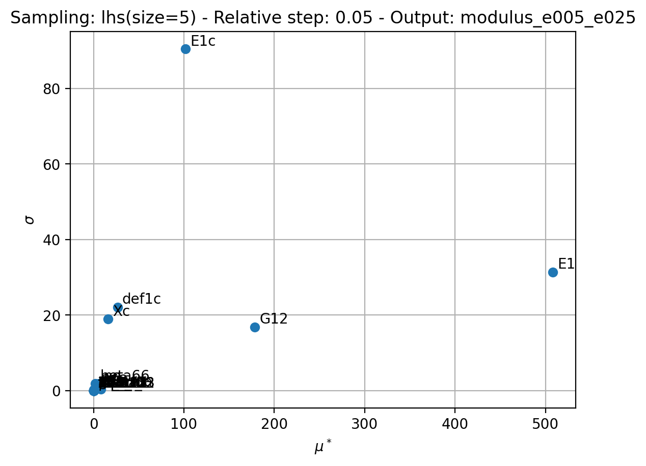
Finally, more details about the sensitivities can be obtained with the \(\sigma\) versus \(\mu^*\) plots. A single output is selected on each plot. The value of \(\sigma\) represents how much the relationship of the output versus an input is non-linear.
| \(cov=5 \%\) |
|---|
 |
 |
Layup \([-60, 0, 60, 0, -60, 60, 60, -60, 0, 60, 0, -60]\)
| \(cov=5 \%\) |
|---|
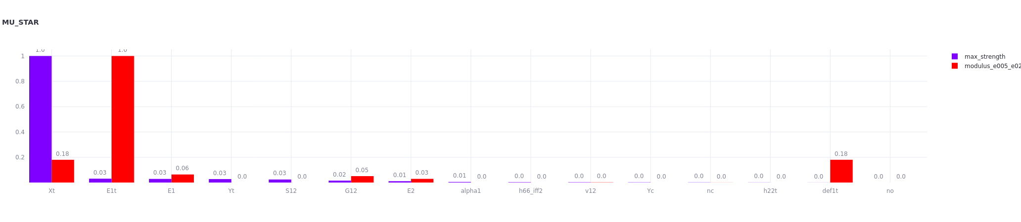 |
Based on the max strength, the most sensitive variables is \(X_t\).
Finally, more details about the sensitivities can be obtained with the \(\sigma\) versus \(\mu^*\) plots.
| \(cov=5 \%\) |
|---|
 |
 |
Layup \([45, -45, 0, 45, -45, -45, 45, 0, -45, 45]\)
| \(cov=5 \%\) |
|---|
 |
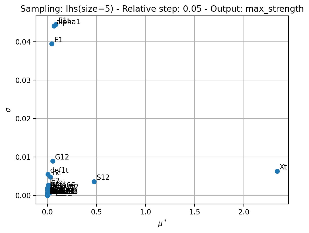
Based on the max strength, the most sensitive variables is \(X_t\) and \(S_{12}\).
Finally, more details about the sensitivities can be obtained with the \(\sigma\) versus \(\mu^*\) plots.
| \(cov=5 \%\) |
|---|
 |
 |
OpfmCube PSC
Layup \([30, 90, -30, 90, -30, -30, 90, -30, 90, 30]\)
| \(cov=5 \%\) |
|---|
 |
| \(cov = 5 \%\) |
|---|
 |
Based on the max strength, the most sensitive variables are \(X_c\), \(S_{12}\), \(E_1\), \(G_{12}\) and \(E_{1c}\).
Finally, more details about the sensitivities can be obtained with the \(\sigma\) versus \(\mu^*\) plots.
| \(cov=5 \%\) |
|---|
 |
 |
Layup \([-60, 0, 60, 0, -60, 60, 60, -60, 0, 60, 0, -60]\)
The same plots are now shown for another layup.
| \(cov=5 \%\) |
|---|
 |
| \(cov=20 \%\) |
|---|
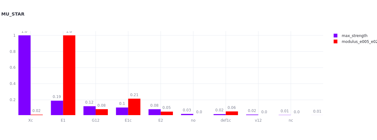 |
We note that the sensitivities are very close for the two parameter spaces. Thus, for this layup, the sensitivities are mostly independent of the width of the distribution around the default input values. Based on the max strength, the most sensitivity variables are \(X_c\), \(E_1\).
TODO: why the variable names are not shown on some plots?
| \(cov=5 \%\) | \(cov=20\%\) |
|---|---|
 |
 |
 |
 |
Layup \([45, -45, 0, 45, -45, -45, 45, 0, -45, 45]\)
| \(cov=5 \%\) |
|---|
 |
| \(cov=20 \%\) |
|---|
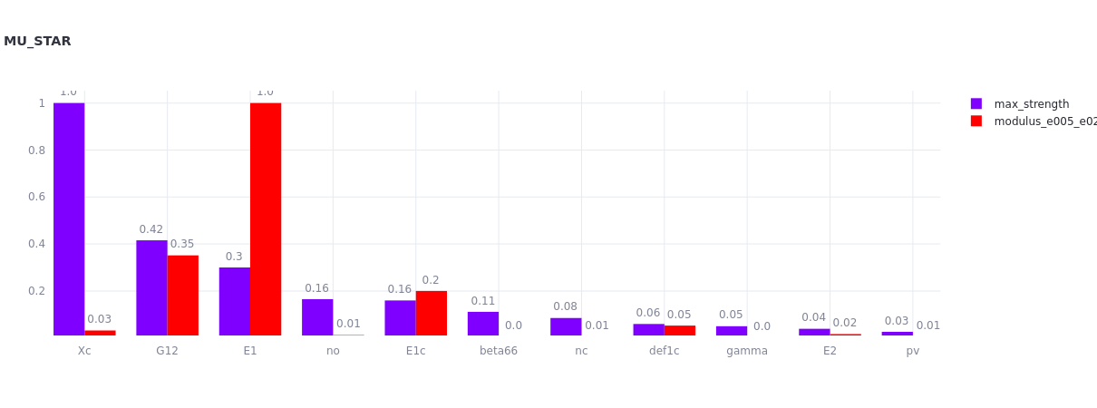 |
Again, the \(\mu^*\) indicator is mostly independent of the two chosen parameter spaces. Based on the max strength, the most sensitivity variables are \(X_c\), \(G_{12}\) and \(E_1\).
| \(cov=5 \%\) | \(cov=20\%\) |
|---|---|
 |
 |
 |
 |
However, the non-linearity magnitude are very different between the two parameter spaces.